The first step is to pre-process models that only specify abundances, to determine the volumes of each element.
Assume that each element has been subjected to enough pressure to compress it down to its liquid density, and no further (i.e., the Coulomb barrier is not being crossed).
Divide the liquid density by the atomic mass to find the number of atoms in a given volume of an element.
Multiply the atoms/volume by the abundance factor, to get the volume.
Knowing the volume of each element, we can determine the average density.
Assuming that the elements are not mixed, and that the densest elements have settled to the bottom, we can then estimate the radii of each elementary layer.
Knowing which elements are present at which depths, the FEA engine can then be invoked, to calculate the force of gravity, given the density of each parcel. From that force, the pressure can be determined, and the model temperature can be checked.
The results for the Anders & Grevesse's numbers are shown in . Note that the element list in the upper panel (which is legible in the 11x17 version) has been re-sorted by liquid density, decreasing from left to right. When no correction factor is applied, we get an average density of 80 kg/m3, which is 17 times lower than the actual density of the Sun (1408 kg/m3). The plot of the radii in the lower panel shows hydrogen occupying all of convective zone and 1/3 of the radiative zone, with helium occupying most of the rest of the volume.
The reason for the inordinately low average density can only be that we have overestimated the volume of the lighter elements. This is no surprise, since the abundances were derived from photons emitted by the outer layer of the Sun. (We would be just as wrong if, on the basis of the composition of the Earth's atmosphere, we concluded that the whole Earth is 78% nitrogen, 21% oxygen, and 1% trace elements.) So we should like to weight the abundances, preferentially decreasing the volume of lighter elements, to get closer to the actual abundances in the whole Sun.1,2 If we apply a linear correction factor, we get results as in Figure 1. This yields 1411 kg/m3.
Figure 1. Abundances with linear correction for mass separation. (See the 11x17 PDF version.)
When we do this, we immediately see two large steps in density. We will suspect that these actually correspond to the known boundaries in the Sun. If, instead of a linear correction factor, we apply a bezier curve to modulate the abundances, we get the results shown in Figure 2. The curve is very slight, but it gets the sharp density changes to match up with known boundaries.
Figure 2. Abundances with bezier correction for mass separation. (See the 11x17 PDF version.)
This seems to be correct, but it yields an overall density of 2767 kg/m3, which is a little less than double the target density of 1408 kg/m3 in the Sun. The discrepancy is to be found in our assumptions. We based our estimates of the average density on the liquid density of each element. But if we revisit the density estimates in the standard model, we see that most of the nickel, all of the iron, and most of the hydrogen are above their liquid densities. (See Figure 3.) If we recalculate the average density cutting these elements in half, 2767 kg/m3 gets reduced to very close to the target density.
Working with Oliver Manuel's numbers, we get different results.
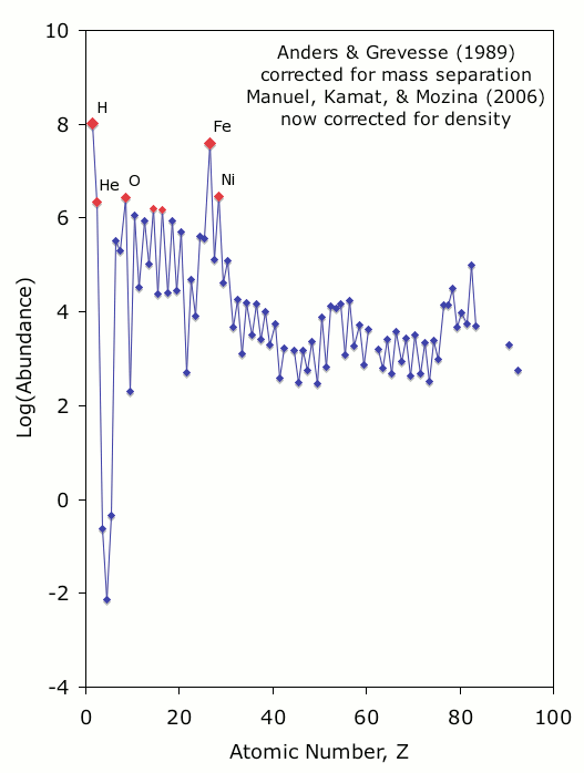
Figure 4. Abundances corrected for mass separation & density, per Manuel, Kamat, & Mozina (2006).
These numbers produce the following results.
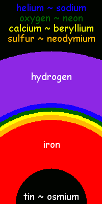
Figure 5. Volumes corrected for mass separation & density, per Manuel, Kamat, & Mozina (2006).